\[\text{Classifier Model}\]

Data Cleaning
1 Remove NaNs
Binary Model
1 Imbalanced Classes
2 Overfitting
3 Precision Recall
4 K-Fold Prediction
Multiclass Prediction

[1]:

import sys; sys.path.insert(1, '../pipeline/lib')
import utils, data_processing

import pandas as pd
import numpy as np

from sklearn.experimental import enable_iterative_imputer
from sklearn.impute import IterativeImputer
from sklearn.neighbors import NearestNeighbors
from sklearn.linear_model import LinearRegression
from sklearn.model_selection import train_test_split
from sklearn.utils import resample

from plotly.offline import init_notebook_mode
init_notebook_mode(connected = True)

import xgboost as xgb

When looking at the boxplot graphs from the 1.FirstAnalysis.ipynb notebook we can see that the behavior of both positive classes - 1 and 2 - are similar. Those are both minority classes so let’s group them and try to create a better binary classification model. This way our model can better both behaviors and we can later use the information from the binary model in our multiclass model.

Data Cleaning¶

[2]:

df_train = pd.read_csv('../../data/train-validation/training-data.csv', index_col = 0)

categorical  = ['Tipo_de_Cultivo','Tipo_de_Solo','Categoria_Pesticida', 'Temporada']
quantitative = ['Estimativa_de_Insetos', 'Semanas_Utilizando', 'Semanas_Sem_Uso']

label = 'dano_na_plantacao'

# Group labels 1 and 2
binary_label = 'dano_na_plantacao_binario'
df_train[binary_label] =  df_train[label].map({0:0,1:1,2:1}).values

# Split features and label
train_labels  = df_train[label].values
train_binary_labels = df_train[binary_label].values
df_train = df_train.iloc[:,1:]

Remove Nans¶

Fill missing values base on the 2.MissingValues.ipynb

[3]:

df_train.columns[df_train.isna().any()]

[3]:

Index(['Semanas_Utilizando'], dtype='object')

[4]:

train_data = data_processing.fill_missing_knn(df_train, 'Semanas_Utilizando')
train_data.isna().any()

[4]:

Estimativa_de_Insetos        False
Tipo_de_Cultivo              False
Tipo_de_Solo                 False
Categoria_Pesticida          False
Doses_Semana                 False
Semanas_Utilizando           False
Semanas_Sem_Uso              False
Temporada                    False
dano_na_plantacao            False
dano_na_plantacao_binario    False
dtype: bool

Binary Model¶

[5]:

train_data[binary_label].value_counts()

[5]:

0    46609
1     9391
Name: dano_na_plantacao_binario, dtype: int64

Since we already have a training-testing dataset (0.75 from original dataset) let’s use 0.2 from train-test dataset for testing.

$ 0.2 :nbsphinx-math:`times `0.75 = 0.15$

This way we can achieve the desired ratio:

Complete dataset 100% -> Training-Testing 75% + Validation 15%

Complete dataset 100% -> Training 75% + Testing 15% + Validation 15%

[6]:

df_train_ohe = data_processing.ohe(train_data, categorical)

X_train, X_test, y_train, y_test = train_test_split(
                                        df_train_ohe.drop(columns = [label, binary_label]),
                                        df_train_ohe[binary_label],
                                        test_size=0.2,
                                        random_state=33)

[7]:

%%time
try:
    xgb_model = xgb.XGBClassifier(objective = 'binary:logistic',
                                  tree_method = 'gpu_hist')
    xgb_model.fit(X_train, y_train)
    print('Training on GPU')
except:
    print('GPU not found!')
    xgb_model = xgb.XGBClassifier(objective = 'binary:logistic')
    xgb_model.fit(X_train, y_train)

preds_xgb = xgb_model.predict(X_test)
preds_xgb_proba = xgb_model.predict_proba(X_test)

Training on GPU
CPU times: user 724 ms, sys: 120 ms, total: 844 ms
Wall time: 696 ms

[8]:

display(utils.Evaluate(y_test, preds_xgb, preds_xgb_proba[:,0], ['0', '1']))

../_images/notebooks_3.MachineLearning_14_0.png

	Accuracy	F1 Score Weighted	ROC AUC
0	0.850357	0.658168	0.193485

Imbalanced classes¶

Let’s deal with the class imbalance problem by upsampling the minority class

[9]:

training_set = X_train.copy()
training_set[binary_label] = y_train

df_minority = training_set[training_set[binary_label] == 1]
df_majority = training_set[training_set[binary_label] == 0]
print('Minority class:',len(df_minority),'\nMajority class:', len(df_majority))

Minority class: 7488
Majority class: 37312

[10]:

# Upsample minority class
df_minority_upsampled = resample(df_minority,
                                 replace=True,
                                 n_samples=46609,
                                 random_state=33)

# Combine majority class with upsampled minority class
df_upsampled = pd.concat([df_majority, df_minority_upsampled])

X_train = df_upsampled.drop(columns = [binary_label]).copy()
y_train = df_upsampled[binary_label].copy()

df_upsampled[binary_label].value_counts().to_frame()

[10]:

	dano_na_plantacao_binario
1	46609
0	37312

The testing subset is still unbalanced!

[11]:

unique, counts = np.unique(y_test, return_counts=True)
print(unique, counts/len(y_test) * 100)

[0 1] [83.00892857 16.99107143]

[12]:

%%time

eval_set = [(X_train, y_train), (X_test, y_test)]

xgb_fit_parameters = dict(
                  eval_metric=["error", "logloss"],
                  eval_set= eval_set,
                  verbose=False
                    )

try:
    xgb_model = xgb.XGBClassifier(objective = 'binary:logistic',
                                  tree_method = 'gpu_hist')
    xgb_model.fit(X_train, y_train, **xgb_fit_parameters)
    print('Training on GPU')
except:
    xgb_model.fit(X_train, y_train, **xgb_fit_parameters)

preds_xgb = xgb_model.predict(X_test)
preds_xgb_proba = xgb_model.predict_proba(X_test)

Training on GPU
CPU times: user 2.71 s, sys: 87.6 ms, total: 2.8 s
Wall time: 840 ms

[13]:

X_train.to_csv('x_train.csv')
y_train.to_csv('y_train.csv')
X_test.to_csv('x_test.csv')
y_test.to_csv('y_test.csv')

[14]:

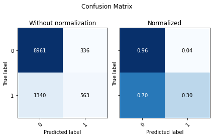
display(utils.Evaluate(y_test, preds_xgb, preds_xgb_proba[:,1], ['0', '1']))

../_images/notebooks_3.MachineLearning_23_0.png

	Accuracy	F1 Score Weighted	ROC AUC
0	0.713036	0.634795	0.79984

Is overfitting occurring?

XGBoost is famous for overfitting, let’s predict on the training data. This way we can see if the model is overfitted the training data and not performing so well on new data.

[15]:

# Predict on training data
preds_xgb_train = xgb_model.predict(X_train)
preds_xgb_proba_train = xgb_model.predict_proba(X_train)

display(utils.Evaluate( df_upsampled[binary_label].values, preds_xgb_train,preds_xgb_proba_train[:,1], ['0', '1']))

../_images/notebooks_3.MachineLearning_25_0.png

	Accuracy	F1 Score Weighted	ROC AUC
0	0.807355	0.802743	0.887432

The training results are better than the testing results, let’s look at whats going on

[16]:

from plotly.subplots import make_subplots
import plotly.graph_objects as go
results = xgb_model.evals_result()
epochs = len(results['validation_0']['error'])
x_axis = list(range(0, epochs))
# plot log loss

fig = make_subplots()
fig.add_trace(go.Scatter(
    x = x_axis,
    y = results['validation_0']['logloss'],
    name = 'Train'
             ))
fig.add_trace(go.Scatter(
    x = x_axis,
    y = results['validation_1']['logloss'],
    name = 'Test'
             ))
fig.update_layout( title = 'log Loss', xaxis_title = 'Epochs', yaxis_title = 'Loss')
fig.show()

Overfitting¶

[17]:

%%time

eval_set = [(X_train, y_train), (X_test, y_test)]

xgb_fit_parameters = dict(
                  eval_metric=["error", "logloss"],
                  eval_set= eval_set,
                  verbose=False
                    )

try:
    xgb_model = xgb.XGBClassifier(objective = 'binary:logistic',
                                  tree_method = 'gpu_hist',
                                  subsample = 0.4,
                                  n_estimators = 1000,
                                  colsample_bytree= 0.8,
                                  learning_rate = 0.0001 )
    xgb_model.fit(X_train, y_train, **xgb_fit_parameters)
    print('Training on GPU')
except:
    xgb_model.fit(X_train, y_train, **xgb_fit_parameters)

preds_xgb = xgb_model.predict(X_test)
preds_xgb_proba = xgb_model.predict_proba(X_test)

display(utils.Evaluate(y_test, preds_xgb, preds_xgb_proba[:,1], ['0', '1']))


results = xgb_model.evals_result()
epochs = len(results['validation_0']['error'])
x_axis = list(range(0, epochs))

fig = make_subplots()
fig.add_trace(go.Scatter(
    x = x_axis,
    y = results['validation_0']['logloss'],
    name = 'Train'
             ))
fig.add_trace(go.Scatter(
    x = x_axis,
    y = results['validation_1']['logloss'],
    name = 'Test'
             ))
fig.update_layout( title = 'log Loss', xaxis_title = 'Iterations', yaxis_title = 'Loss')
fig.show()

Training on GPU

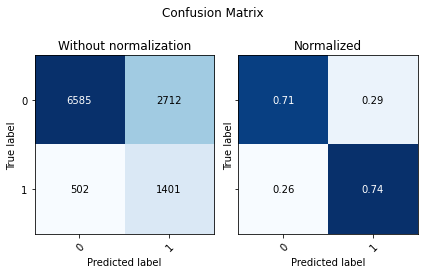
../_images/notebooks_3.MachineLearning_29_1.png

	Accuracy	F1 Score Weighted	ROC AUC
0	0.684821	0.619654	0.802329

CPU times: user 11 s, sys: 169 ms, total: 11.2 s
Wall time: 5.52 s

Precision Recall¶

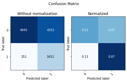
Looking at the not normalized Confusion Matrix we see that our model identified a lot more of our minority classes, this comes with a downside, we are predicting a lot of false positives, and since our negative (0) class is much larger, we end up with lower accuracy.

By default models use a threshold of 0.5, we can look at the precision and recall and see if it is worth using another value. This also depends on what is important for the model, do we want to find all the minority classes even if we have lower precision, or having a higher precision and being sure the prediction of the minority class is right is better?

[18]:

fig = utils.plot_precision_recall(y_test, preds_xgb_proba[:,1])
fig.show()

[19]:

threshold = 0.49
predictions = (preds_xgb_proba[:,1] > threshold).astype(int)

display(utils.Evaluate(y_test, predictions, preds_xgb_proba[:,1], ['0', '1']))

../_images/notebooks_3.MachineLearning_33_0.png

	Accuracy	F1 Score Weighted	ROC AUC
0	0.589018	0.550128	0.802329

Ok so now what? We have a binary classification model that’s not what we wanted!

As we saw in the initial analysis the labels 1 and 2 seem very similar. So it’s easier for our model to predict Damage (1/2) or No Damage (0) but not so trivial to differ class 1 from 2.

Let’s try to use the positive predicted class for our multi-class classification, this way our class imbalance is not so big.

K-Fold prediction¶

Here we want to use predicted data to train another model, but it would be unfair if our predicted data was also used from training. So what we can do a k-fold cross-validation prediction, this way we can prediction on the whole training-testing dataset without predicting on training data.

k-fold cross-validation prediction is when we divide the dataset into k subsets and use k-1 to train the model and prediction holdout group. This is done k times alternating between subsets so that we never predict on training data and we can predict the complete dataset.

It’s important to remember that our training data also goes through some transformation - fill in missing values, one hot encoding, and upscaling -we can apply these transformations on our prediction data, but we can’t apply to upscale.

[20]:

df_train = df_train.reset_index(drop = True)

# Remove labels to predict missing values
cv_data = data_processing.fill_missing_knn(df_train.drop(columns = [label, binary_label]), 'Semanas_Utilizando')

# Insert back labels to train
cv_data[binary_label] = df_train[binary_label]
cv_data[label] = df_train[label]
cv_data = data_processing.ohe(cv_data, categorical).reset_index(drop = True)

cv_data.head(2)

[20]:

	Estimativa_de_Insetos	Doses_Semana	Semanas_Utilizando	Semanas_Sem_Uso	dano_na_plantacao_binario	dano_na_plantacao	Tipo_de_Cultivo_1	Tipo_de_Solo_1	Categoria_Pesticida_2	Categoria_Pesticida_3	Temporada_2	Temporada_3
0	2267	20	55.0	0	1	1	0	1	0	1	0	0
1	984	25	23.0	13	0	0	0	1	1	0	0	1

[21]:

df_with_prediction = cv_data.copy()
df_with_prediction.insert(cv_data.shape[1], 'binary_prediction_proba', 0)
df_with_prediction.insert(cv_data.shape[1], 'binary_prediction', 0)

[22]:

from sklearn.model_selection import KFold

# 5 CrossValidation Splits
kf = KFold(n_splits=5)
kf.get_n_splits(cv_data)

xbg_args = dict(
           objective = 'binary:logistic',
           tree_method = 'gpu_hist',
           subsample = 0.4,
           n_estimators = 1000,
           colsample_bytree= 0.8,
           learning_rate = 0.0001
                )

for i, (train_index, test_index) in enumerate(kf.split(cv_data)):
    print(f'{i+1}/{kf.n_splits}: TRAIN: {len(train_index)} - TEST: {len(test_index)} ')

    cv_train = cv_data.iloc[train_index]

    X = cv_data.drop(columns = [binary_label, label])
    X_test = X.iloc[test_index]

    # Upsample data
    print('Upsampling Data ...')
    df_minority = cv_train[cv_train[binary_label] == 1]
    df_majority = cv_train[cv_train[binary_label] == 0]
    n_upsample = len(df_majority)

    df_minority_upsampled = resample(df_minority,
                                     replace=True,
                                     n_samples=n_upsample,
                                     random_state=33)

    # Combine majority class with upsampled minority class
    df_upsampled = pd.concat([df_majority, df_minority_upsampled])

    X_train = df_upsampled.drop(columns = [binary_label, label]).copy()
    y_train = df_upsampled[binary_label].copy()

    # ML Model
    print('Training Model ...')
    xgb_model = xgb.XGBClassifier( **xbg_args )
    xgb_model.fit(X_train, y_train, verbose=False)

    print('Predicting ...\n')

    # Predict Probability
    proba = xgb_model.predict_proba(X_test)[:,1]
    df_with_prediction.iloc[test_index, -1] = proba

print('Done!')

1/5: TRAIN: 44800 - TEST: 11200
Upsampling Data ...
Training Model ...
Predicting ...

2/5: TRAIN: 44800 - TEST: 11200
Upsampling Data ...
Training Model ...
Predicting ...

3/5: TRAIN: 44800 - TEST: 11200
Upsampling Data ...
Training Model ...
Predicting ...

4/5: TRAIN: 44800 - TEST: 11200
Upsampling Data ...
Training Model ...
Predicting ...

5/5: TRAIN: 44800 - TEST: 11200
Upsampling Data ...
Training Model ...
Predicting ...

Done!

[23]:

import joblib
#save model
filename = 'xgb_binary_classifier.xgb'
joblib.dump(xgb_model, filename)

# #load saved model
# xgb = joblib.load(filename)

[23]:

['xgb_binary_classifier.xgb']

[24]:

threshold = 0.48

# Get classes from prediction probability
df_with_prediction['binary_prediction'] = (df_with_prediction['binary_prediction_proba'] >
                                           threshold).astype(int)

# Evaluate
fig = utils.plot_precision_recall(df_with_prediction[binary_label],
                                  df_with_prediction['binary_prediction_proba'].values)
fig.show()

display(utils.Evaluate(df_with_prediction[binary_label],
                       (df_with_prediction['binary_prediction_proba'] > threshold).astype(int),
                       df_with_prediction['binary_prediction_proba'],
                       ['0', '1']))

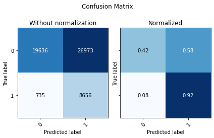
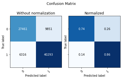
../_images/notebooks_3.MachineLearning_41_1.png

	Accuracy	F1 Score Weighted	ROC AUC
0	0.505214	0.485432	0.800882

[25]:

df_wPred = df_with_prediction.drop(columns = ['binary_prediction_proba', binary_label])

MultiClass Prediction¶

Now from our predicted dataframe we will split into train and testing

[26]:

X_train, X_test, y_train, y_test = train_test_split(
                                                    df_wPred.drop(columns = [label]), # X
                                                    df_wPred[label].values,           # Y
                                                    test_size=0.2,
                                                    random_state=33
                                                    )

train_df = X_train.copy(); train_df[label] = y_train
test_df  = X_test.copy(); test_df[label] = y_test

[27]:

pp_train_df = train_df[train_df['binary_prediction'] == 1] # Positive predicted
np_train_df = train_df[train_df['binary_prediction'] == 0] # Negative predicted

pp_test_df = test_df[test_df['binary_prediction'] == 1] # Positive predicted
np_test_df = test_df[test_df['binary_prediction'] == 0] # Negative predicted

[28]:

print('Positive Predicted Class Count')
display(pp_train_df[label].value_counts().to_frame() )

print('\n\n\nNegative Predicted Class Count')
display(np_train_df[label].value_counts().to_frame() )

Positive Predicted Class Count

	dano_na_plantacao
0	21570
1	5783
2	1146




Negative Predicted Class Count

	dano_na_plantacao
0	15725
1	531
2	45

Looking at both label value counts we can see in the positive predicted subset we were able to remove most of the 0 Label - we only kept 13% of the total. But we kept 50% of class 1 and 70% from class 2.

[29]:

pp_labels = pp_train_df[label].values

w_array = np.zeros(pp_labels.shape)

for l in np.unique(pp_labels):
    w_array[pp_labels == l] = 1- len(pp_labels[pp_labels == l])/len(pp_labels)

display(pd.DataFrame(zip(w_array,pp_labels), columns = ['Weights', 'Labels']).groupby('Labels').mean())

	Weights
Labels
0	0.243131
1	0.797081
2	0.959788

[30]:

%%time


pp_train_X = pp_train_df.drop(columns = [label, 'binary_prediction'])
pp_train_y = pp_train_df[label].values

pp_test_X = pp_test_df.drop(columns = [label, 'binary_prediction'])
pp_test_y = pp_test_df[label].values

xgb_model = xgb.XGBClassifier(objective = 'bjective=multi:softmax',
                              tree_method = 'gpu_hist')
xgb_model.fit(pp_train_X, pp_train_y,  sample_weight = w_array)

preds_xgb = xgb_model.predict(pp_test_X)
preds_xgb_proba = xgb_model.predict_proba(pp_test_X)

preds_xgb = xgb_model.predict(pp_test_X)
preds_xgb_proba = xgb_model.predict_proba(pp_test_X)

display(utils.Evaluate(pp_test_y, preds_xgb, preds_xgb_proba, ['0', '1','2']))

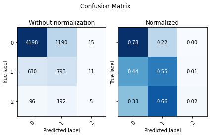
../_images/notebooks_3.MachineLearning_50_0.png

	Accuracy	F1 Score Weighted	ROC AUC
0	0.700701	0.427779	0.720175

CPU times: user 16.4 s, sys: 432 ms, total: 16.8 s
Wall time: 1.66 s

[31]:

#save model
filename = 'xgb_multilabel_classifier.xgb'
joblib.dump(xgb_model, filename)

[31]:

['xgb_multilabel_classifier.xgb']

[32]:

pd.DataFrame(list(zip(preds_xgb_proba[:,0],preds_xgb_proba[:,1],preds_xgb_proba[:,2],  preds_xgb)),
             columns= ['Proba 0','Proba 1', 'Proba 2','Class Pred'])

[32]:

	Proba 0	Proba 1	Proba 2	Class Pred
0	0.101900	0.549280	0.348820	1
1	0.226323	0.400158	0.373519	1
2	0.916526	0.076652	0.006822	0
3	0.333894	0.529902	0.136205	1
4	0.323089	0.662145	0.014766	1
...	...	...	...	...
7125	0.349980	0.581073	0.068946	1
7126	0.863426	0.134723	0.001851	0
7127	0.580020	0.412889	0.007091	0
7128	0.635819	0.314860	0.049321	0
7129	0.575227	0.171962	0.252811	0

7130 rows × 4 columns

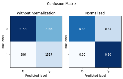
Remember, here we are just working with a subset from our dataframe which the binary classifier predicted a positive class (1). So we can adjust the threshold to try to bring our confusion matrix to the right (1 or 2), any false negatives we have here is not a problem since it’s a small percentage from the complete data.

[33]:

display(utils.Evaluate(pp_test_y, preds_xgb, preds_xgb_proba, ['0', '1','2']))

../_images/notebooks_3.MachineLearning_54_0.png

	Accuracy	F1 Score Weighted	ROC AUC
0	0.700701	0.427779	0.720175

[34]:

try:
    np_test_df.insert(np_test_df.shape[1], 'MultiClass_Prediction', 0 )
    pp_test_df.insert(pp_test_df.shape[1], 'MultiClass_Prediction', preds_xgb )
    pp_test_df.insert(pp_test_df.shape[1], 'MultiClass_ProbaPrediction_0', preds_xgb_proba[:,0] )
    pp_test_df.insert(pp_test_df.shape[1], 'MultiClass_ProbaPrediction_1', preds_xgb_proba[:,1] )
    pp_test_df.insert(pp_test_df.shape[1], 'MultiClass_ProbaPrediction_2', preds_xgb_proba[:,2] )
except ValueError:
    np_test_df['MultiClass_Prediction'] = 0
    pp_test_df['MultiClass_Prediction'] = preds_xgb

    pp_test_df['MultiClass_ProbaPrediction_0'] = preds_xgb_proba[:,0]
    pp_test_df['MultiClass_ProbaPrediction_1'] = preds_xgb_proba[:,1]
    pp_test_df['MultiClass_ProbaPrediction_2'] = preds_xgb_proba[:,2]

[35]:

df_evaluate = pd.concat([np_test_df, pp_test_df])

[36]:

df_evaluate['MultiClass_ProbaPrediction_0'] = df_evaluate['MultiClass_ProbaPrediction_0'].fillna(1)
df_evaluate['MultiClass_ProbaPrediction_1'] = df_evaluate['MultiClass_ProbaPrediction_1'].fillna(0)
df_evaluate['MultiClass_ProbaPrediction_2'] = df_evaluate['MultiClass_ProbaPrediction_2'].fillna(0)

[37]:

pred_proba = df_evaluate[['MultiClass_ProbaPrediction_0',
                          'MultiClass_ProbaPrediction_1',
                          'MultiClass_ProbaPrediction_2']].values

[38]:

display(utils.Evaluate(df_evaluate[label],
                       df_evaluate['MultiClass_Prediction'],
                       pred_proba,
                       ['0', '1','2']))

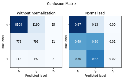
../_images/notebooks_3.MachineLearning_59_0.png

	Accuracy	F1 Score Weighted	ROC AUC
0	0.795268	0.445987	0.784457

Scicrop documentation