\[\text{Data Analysis}\]
This notebook is our first look at the data. Here we will try to extract information that can be useful for our model later, we will look at our label behaves when grouping the data in different ways.
1. Class Balance
2. Missing Data
3. Features Analysis
3.1 Quantitative Features
3.2 Categorical and Quantitative Grouping
4. Clustering
Class Balance
|
Count [%] |
| dano_na_plantacao |
|
| 0 |
83.230357 |
| 1 |
14.091071 |
| 2 |
2.678571 |
Identificador_Agricultor 0
Estimativa_de_Insetos 0
Tipo_de_Cultivo 0
Tipo_de_Solo 0
Categoria_Pesticida 0
Doses_Semana 0
Semanas_Utilizando 5690
Semanas_Sem_Uso 0
Temporada 0
dano_na_plantacao 0
dtype: int64
Missing Data
|
Estimativa_de_Insetos |
Tipo_de_Cultivo |
Tipo_de_Solo |
Categoria_Pesticida |
Doses_Semana |
Semanas_Utilizando |
Semanas_Sem_Uso |
Temporada |
dano_na_plantacao |
| count |
50310.000000 |
50310.000000 |
50310.000000 |
50310.000000 |
50310.000000 |
50310.000000 |
50310.000000 |
50310.000000 |
50310.000000 |
| mean |
1399.919579 |
0.283542 |
0.457364 |
2.270443 |
25.862353 |
28.651719 |
9.512025 |
1.896263 |
0.193977 |
| std |
851.705790 |
0.450722 |
0.498184 |
0.465177 |
15.584169 |
12.429610 |
9.903693 |
0.703317 |
0.457630 |
| min |
150.000000 |
0.000000 |
0.000000 |
1.000000 |
0.000000 |
0.000000 |
0.000000 |
1.000000 |
0.000000 |
| 25% |
731.000000 |
0.000000 |
0.000000 |
2.000000 |
15.000000 |
20.000000 |
0.000000 |
1.000000 |
0.000000 |
| 50% |
1212.000000 |
0.000000 |
0.000000 |
2.000000 |
20.000000 |
28.000000 |
7.000000 |
2.000000 |
0.000000 |
| 75% |
1898.000000 |
1.000000 |
1.000000 |
3.000000 |
40.000000 |
37.000000 |
16.000000 |
2.000000 |
0.000000 |
| max |
4097.000000 |
1.000000 |
1.000000 |
3.000000 |
95.000000 |
67.000000 |
50.000000 |
3.000000 |
2.000000 |
<ipython-input-7-cded8ad30d30>:2: UserWarning:
Boolean Series key will be reindexed to match DataFrame index.
|
Estimativa_de_Insetos |
Tipo_de_Cultivo |
Tipo_de_Solo |
Categoria_Pesticida |
Doses_Semana |
Semanas_Utilizando |
Semanas_Sem_Uso |
Temporada |
dano_na_plantacao |
| count |
0.0 |
0.0 |
0.0 |
0.0 |
0.0 |
0.0 |
0.0 |
0.0 |
0.0 |
| mean |
NaN |
NaN |
NaN |
NaN |
NaN |
NaN |
NaN |
NaN |
NaN |
| std |
NaN |
NaN |
NaN |
NaN |
NaN |
NaN |
NaN |
NaN |
NaN |
| min |
NaN |
NaN |
NaN |
NaN |
NaN |
NaN |
NaN |
NaN |
NaN |
| 25% |
NaN |
NaN |
NaN |
NaN |
NaN |
NaN |
NaN |
NaN |
NaN |
| 50% |
NaN |
NaN |
NaN |
NaN |
NaN |
NaN |
NaN |
NaN |
NaN |
| 75% |
NaN |
NaN |
NaN |
NaN |
NaN |
NaN |
NaN |
NaN |
NaN |
| max |
NaN |
NaN |
NaN |
NaN |
NaN |
NaN |
NaN |
NaN |
NaN |
|
Estimativa_de_Insetos |
Tipo_de_Cultivo |
Tipo_de_Solo |
Categoria_Pesticida |
Doses_Semana |
Semanas_Utilizando |
Semanas_Sem_Uso |
Temporada |
dano_na_plantacao |
| count |
50310.000000 |
50310.000000 |
50310.000000 |
50310.000000 |
50310.000000 |
50310.000000 |
50310.000000 |
50310.000000 |
50310.000000 |
| mean |
1399.919579 |
0.283542 |
0.457364 |
2.270443 |
25.862353 |
28.651719 |
9.512025 |
1.896263 |
0.193977 |
| std |
851.705790 |
0.450722 |
0.498184 |
0.465177 |
15.584169 |
12.429610 |
9.903693 |
0.703317 |
0.457630 |
| min |
150.000000 |
0.000000 |
0.000000 |
1.000000 |
0.000000 |
0.000000 |
0.000000 |
1.000000 |
0.000000 |
| 25% |
731.000000 |
0.000000 |
0.000000 |
2.000000 |
15.000000 |
20.000000 |
0.000000 |
1.000000 |
0.000000 |
| 50% |
1212.000000 |
0.000000 |
0.000000 |
2.000000 |
20.000000 |
28.000000 |
7.000000 |
2.000000 |
0.000000 |
| 75% |
1898.000000 |
1.000000 |
1.000000 |
3.000000 |
40.000000 |
37.000000 |
16.000000 |
2.000000 |
0.000000 |
| max |
4097.000000 |
1.000000 |
1.000000 |
3.000000 |
95.000000 |
67.000000 |
50.000000 |
3.000000 |
2.000000 |
<ipython-input-9-cded8ad30d30>:2: UserWarning:
Boolean Series key will be reindexed to match DataFrame index.
|
Estimativa_de_Insetos |
Tipo_de_Cultivo |
Tipo_de_Solo |
Categoria_Pesticida |
Doses_Semana |
Semanas_Utilizando |
Semanas_Sem_Uso |
Temporada |
dano_na_plantacao |
| count |
0.0 |
0.0 |
0.0 |
0.0 |
0.0 |
0.0 |
0.0 |
0.0 |
0.0 |
| mean |
NaN |
NaN |
NaN |
NaN |
NaN |
NaN |
NaN |
NaN |
NaN |
| std |
NaN |
NaN |
NaN |
NaN |
NaN |
NaN |
NaN |
NaN |
NaN |
| min |
NaN |
NaN |
NaN |
NaN |
NaN |
NaN |
NaN |
NaN |
NaN |
| 25% |
NaN |
NaN |
NaN |
NaN |
NaN |
NaN |
NaN |
NaN |
NaN |
| 50% |
NaN |
NaN |
NaN |
NaN |
NaN |
NaN |
NaN |
NaN |
NaN |
| 75% |
NaN |
NaN |
NaN |
NaN |
NaN |
NaN |
NaN |
NaN |
NaN |
| max |
NaN |
NaN |
NaN |
NaN |
NaN |
NaN |
NaN |
NaN |
NaN |
Features Analysis
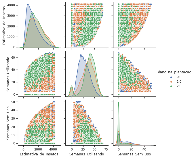
Quantitative Features
By separating our label by color, we can see here that there is no easy separation of the classes just by looking at two features at a time.
Categorical and Quantitative Grouping
We can notice here that the label 1 and 2 are very simmilar for most of the grouping done. Let’s try to combine those two and see if we can find any paterns.
|
Estimativa_de_Insetos |
Tipo_de_Cultivo |
Tipo_de_Solo |
Categoria_Pesticida |
Doses_Semana |
Semanas_Utilizando |
Semanas_Sem_Uso |
Temporada |
dano_na_plantacao_binario |
| dano_na_plantacao |
|
|
|
|
|
|
|
|
|
| 0.0 |
1218.511538 |
1.0 |
0.213878 |
2.421305 |
21.488297 |
26.905136 |
6.412207 |
1.900505 |
0 |
| 1.0 |
1633.192933 |
1.0 |
0.354459 |
2.628716 |
18.839035 |
32.844644 |
2.380258 |
1.885586 |
1 |
| 2.0 |
1561.723785 |
1.0 |
0.427110 |
2.601023 |
21.470588 |
32.984655 |
0.820972 |
1.884910 |
1 |
Clustering
Now we can try our higher dimensions clustering and see if we get any segregation of the labels
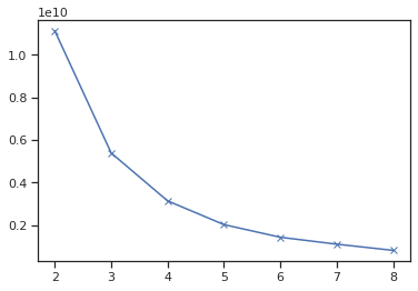
Let’s try different numbers of clusters and use the elbow method to find the optimal number. To determine the optimal number of clusters, we have to select the value of k at the “elbow” ie the point after which the distortion/inertia start decreasing in a linear fashion.
In this case, it looks like the optimal value is k = 4. Let’s look at the clusters and see if there is any segregation done by the unsupervised algorithm.
|
|
Identificador_Agricultor |
| Cluster |
dano_na_plantacao |
|
| 0 |
0.0 |
9066 |
| 1.0 |
2274 |
| 2.0 |
445 |
| 1 |
0.0 |
15442 |
| 1.0 |
1192 |
| 2.0 |
205 |
| 2 |
0.0 |
3487 |
| 1.0 |
1522 |
| 2.0 |
221 |
| 3 |
0.0 |
13891 |
| 1.0 |
2101 |
| 2.0 |
464 |
|
|
Identificador_Agricultor |
| Cluster |
dano_na_plantacao_binario |
|
| 0 |
0 |
9066 |
| 1 |
2719 |
| 1 |
0 |
15442 |
| 1 |
1397 |
| 2 |
0 |
3487 |
| 1 |
1743 |
| 3 |
0 |
13891 |
| 1 |
2565 |
Even after trying to clusters into subgroups by features, there is no significant segregation of the labels. It seems like unsupervised learning won’t help us here.